Tutorial 3: MapReduce

How to use this tutorial

• This tutorial is also available in Jupyter notebook format. To access and run the Jupyter notebook version of the tutorial, please sign up for free developer access by following instructions at https://github.com/juliustechco/juliusgraph.
• Additional resources (video demos & blogs) are available at http://juliustech.co.
• To report bugs or request new features, please raise an issue here. To schedule a live demo, please go to http://juliustech.co. Please check out this FAQ page or email us at info@juliustech.co for other general inquiries.
• This tutorial is copyrighted by Julius Technologies, its use is governed by the terms of use.

Introduction

In this tutorial, we use Julius RuleDSL to build a generic MapReduce pipeline, and illustrate the benefits of Julius' high order rules.

MapReduce is a common pipeline pattern which is often used for processing big data sets in parallel with multiple computers/workers. The MapReduce pipeline is a defining feature in some of the most popular data platforms, such as Hadoop.

In this tutorial, we explain how to build a generic and re-usable MapReduce pipeline using a few simple rules in Julius' low-code declarative RuleDSL, as opposed to writing excessive amounts of code in traditional programming languages.

The MapReduce pipeline is composed of three main steps:

• map: a common map function is applied to every input data batch.
• shuffle: workers redistribute the map output based on certain key values such that all data with the same key value is shipped to the same worker.
• reduce: each worker then processes the results for its subset of keys by applying a reduce function. These reduced results are then collated as the final result.

The following image shows the generic MapReduce steps for the problem of counting the number of occurrences of words in a large collection of documents, which is given in the original Hadoop paper. This word count example is often used to illustrate the MapReduce pipeline. We will replicate this example while building a generic MapReduce pipeline in the Julius RuleDSL from scratch.

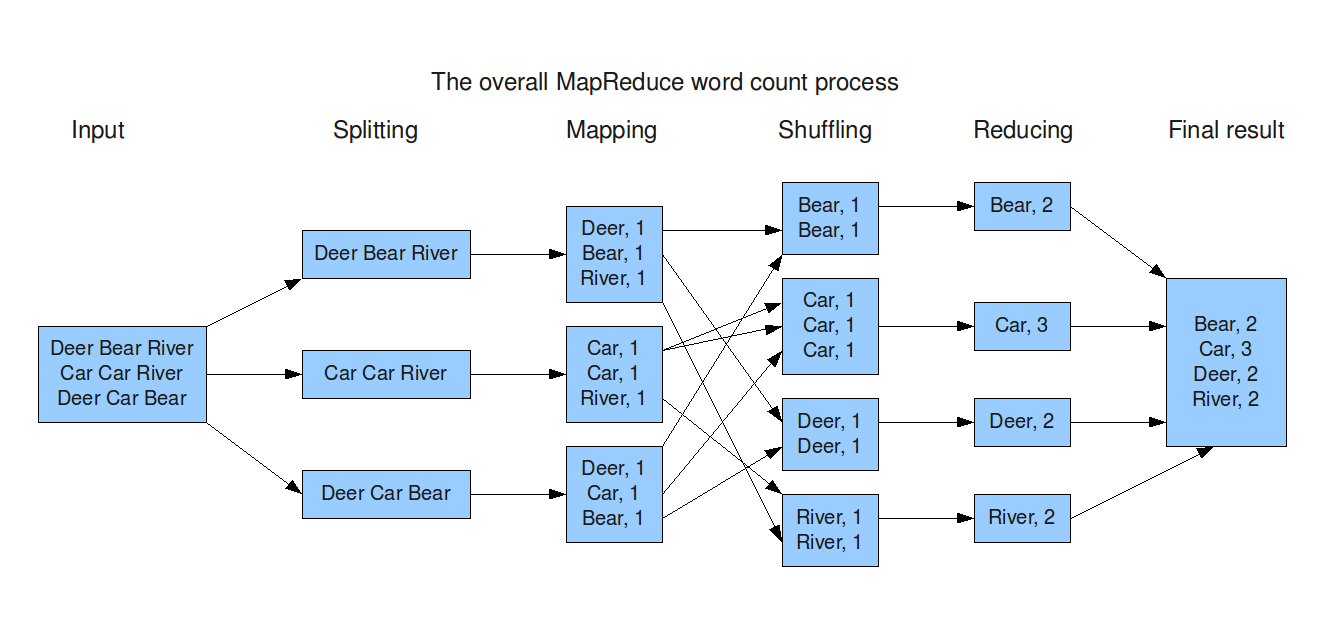
The MapReduce input data is a collection of data batches. The creation of data batches has to be done before the MapReduce pipeline (as in the Splitting stage in the diagram above). For example, if the original data is a single large data file, it has to be split into multiple batches of smaller files before feeding into the MapReduce process.

The goal of this tutorial is to construct a generic mapreduce rule whose mapper, shuffler and reducer operators can be customized by the user. Even though the word count problem itself is trivial, we will implement the pipeline in a generic fashion so that it can be re-used for any MapReduce problems.

The readers are referred to the quick start tutorial for the basic concepts and syntax of the RuleDSL and Atom. But for completeness, we give a brief explanation of the rule syntax and graph execution here.

A rule in RuleDSL has the following syntax:

RuleDSL.@addrules namespace begin
    rulename(rulearg1::Type1, rulearg2::Type2, ...) = begin
        # additional code here transforming ruleargs to atom args and dependent args
        AtomName[atomarg1, atomarg2...](deprule1(depargs1...), deprule2(depargs2...), ...)
    end
end

The RuleDSL.@addrules is a macro used for processing the RuleDSL. It takes a namespace parameter and a set of rule declarations. The rule namespace helps organize the rules into related groups, and avoid name clashes. A rule in the RuleDSL is an instruction to create certain nodes in the computational graph. When the Julius GraphEngine processes a rule, it creates a node from the rule in the computational graph, and then recursively adds the dependent nodes to the graph according to the dependent rules specified in deprule1, deprule2 etc. The AtomName[atomarg1, atomarg2...] syntax defines an Atom object, which is used to process the data from the node's dependency.

As you can now appreciate, graph programming is quite different from traditional programming. Instead of writing imperative functions, we declare the logic and dependencies using rules, then let the Graph Engine create the application or systems as computational DAGs for us. That is why the amount of code required in graph programming is far less than traditional programming languages, since most of the boilerplate code for the program's flow control is automated away.

The generic mapreduce rule should include three stages: mapper, shuffler and reducer, so it should look like:

RuleDSL.@addrules mr begin
    mapreduce(
        batches::Vector{RuleDSL.NodeRef},
        mapper::RuleDSL.NodeRef,
        shuffler::RuleDSL.NodeRef,
        reducer::RuleDSL.NodeRef
    ) = begin
        # ... rule definition goes here ...
    end
end

The RuleDSL.NodeRef is a data structure that refers to another node in the graph. In Julius, every node is created by a specific rule, so that a dependency on another node can also be understood as a dependency on its underlying rule. A rule with a RuleDSL.NodeRef parameter, like the mapreduce rule above, is called a high order rule, as it defines a generic pattern whose behavior depends on other rules. The high order rule is extremely powerful in defining abstract and high level logic and behaviors. Furthermore, a high order rule can be passed as parameter to another rule, creating even higher order rules. The ability to nest high order rules is one of the reasons why the RuleDSL is both low-code and expressive. The high order rule is similar in spirit to the high order functions in functional programming, which we will discuss in more detail at the end of this tutorial.

We now proceed to implement the MapReduce pipeline as depicted in the diagram above using the Julius RuleDSL.

2. Generic Map/Reduce

2.1 Mapping

In the mapping step of the word count example, a batch of data is just a String such as "Mary has a lamb", which is converted into a Vector of Pairs: ["Mary" => 1, "has" => 1, "a" => 1, "lamb" => 1], where each entry represents one occurrence of a given word. At the shuffle stage, the vector is split by a key value, which is the word itself in the above diagram. Then all the pairs for the same keyword are sent to a single node where they are concatenated to form a single vector. Finally at the reducer stage, the total occurrence of each key word is deduced by simply counting their occurrences in the vector.

Given that the logic in the word count example is simple, we use a generic ApplyFn atom that is provided as part of the DataScience package, which can take any Julia function as an argument, so that we don't have to define many Atom types for every stage of the MapReduce process. The ApplyFn source code is listed below, which inherits from the abstract base type Datom and implements a generic method fwddata!, which will be called by the Julius Graph Engine at runtime to process data at individual nodes.

import GraphEngine.RuleDSL: fwddata!

struct ApplyFn <: RuleDSL.Datom
    fn::Any # can be a function or any object with a callable method defined
    params::Tuple # the first few arguments of `fn`

    ## this inner constructor captures `params` as a Tuple
    ApplyFn(fn::Any, params::Any...) = new(fn, params)
end

fwddata!(self::ApplyFn, xs::Any...) = [self.fn(self.params..., xs...)]

Using the generic DataScience.ApplyFn Atom, the mapper rule for word count example can be written as:

using GraphEngine: RuleDSL, GraphVM
using DataScience: ApplyFn
using AtomExt

wordmap(words::String) = [k => 1 for k in split(words)]

RuleDSL.@addrules mr begin
    mapper(batch::RuleDSL.NodeRef, mapfun::Function) = ApplyFn[mapfun](batch...)
end

The GraphEngine.RuleDSL and GraphEngine.GraphVM modules have to be included in order to use the RuleDSL to create and run computational graphs.

The dependency of this rule is simply given as batch..., which specifies that the node represented by the batch parameter is a dependency. The three dot syntax ... designates dynamic dependencies from a NodeRef parameter or variable. At runtime, the Julius GraphEngine first converts the ApplyFn[mapfun] specification to a call to the constructor of ApplyFn(mapfun). Then, the fwddata! method of the ApplyFn atom object is called to process the data from its input node specified by the batch parameter, which in turn calls the underlying mapfun function.

The mapper rule above takes a single RuleDSL.NodeRef as an argument, as it only applies to an individual batch. However, the mapreduce rule needs to process all the mapper results from all the batches. So, how do we make that information available to the mapreduce rule? We could create a collection of mapper rules as Vector{NodeRef} then pass it into the mapreduce rule:

mappers = RuleDSL.@ref(mr.mapper(batch, mapfun) for batch in batches)
mr = RuleDSL.@ref mr.mapreduce(batches, mappers, shufflers, reducers)

where the batches is a Vector{RuleDSL.NodeRef} representing the collection of input batches. However, this approach would require us to also create vectors of shufflers and reducers, thus putting too much burden on the user to ensure their consistency. By observing that the first argument of the mapper rule is its input data batch and that the same mapper rule should be applied to all batch inputs, we instead choose to drop the first argument in the mapper rule before passing it as an argument to the mapreduce rule, such that:

mapper = RuleDSL.@ref mr.mapper(mapfun)
mr = RuleDSL.@ref mr.mapreduce(batches, mapper, shuffler, reducer)

Inside the mapreduce rule, the first argument is added back for every data batch using the following prepend function, to recover the full form of the mapper rule:

prepend(ref::RuleDSL.NodeRef, firstarg::Any) = RuleDSL.NodeRef(ref.ns, ref.name, (firstarg, ref.params...), ref.meta)

prepend (generic function with 1 method)

The advantages of dynamically inserting the first parameter in the mapreduce rule are the following:

• First it is more readable and clear in that we only need the overall rule logic, but not its first argument that specifies a particular batch input.
• Secondly it is less error prone, as the mappers are created inside the mapreduce rule by inserting the right batch as its first parameter, making it fully consistent with the batch input parameter. We will apply the same trick for shuffler and reducer later.

We follow the convention that variables starting with an underscore all reference to those partial rules without its first parameter, making it clear that they shall only be used as parameters to other rules.

Let's test our mapping rule to see how it works. We have to define the input data batches first. For this word count example, we can simply use the ApplyFn atom with the identity function to return a rule argument, such that:

@addrules mr begin
    batch(s::Any) = ApplyFn[identity, s]()
end

# some input data
sentences = ("Deer Bear River", "Car Car River", "Deer Car Bear")
batches   = RuleDSL.@ref(mr.batch(s) for s in sentences)
_mapper    = RuleDSL.@ref mr.mapper(wordmap)

# prepend returns a new `NodeRef` such that `mappers` is of `Vector{NodeRef}` type
mappers = [prepend(_mapper, batch) for batch in batches]

# create a local graph, provide the node references and calculate
config = RuleDSL.Config()
gs1 = GraphVM.createlocalgraph(config, RuleDSL.GenericData())
GraphVM.calcfwd!(gs1, Set(mappers));

We have now created a computational graph for the mapper and executed it. How do we see the results? Julius provides an easy-to-use web UI for users to navigate and visualize the resulting data and logic in the graph. The following code block starts a local server so that the web UI can retrieve the resulting graph data, and it also overrides the RuleDSL.nodelabel method to customize the information displayed on the graph node.

using GraphIO

# a container of graphs
gss = Dict{String,RuleDSL.AbstractGraphState}()

# used for WebUI display purposes
port = GraphVM.drawdataport()
@async GraphVM.startresponder(gss, port);

# override node label display
import GraphEngine.RuleDSL: nodelabel
function nodelabel(gs::RuleDSL.AbstractGraphState, ref::RuleDSL.NodeRef)
    shortrepr(x::Vector; sep=", ") = "["*join(shortrepr.(x), sep)*"]"
    shortrepr(p::Pair; sep="=>") = shortrepr(p.first) * sep * shortrepr(p.second)
    shortrepr(p::Dict; sep=", ") = "{" * join(shortrepr.(collect(p)), sep) * "}"
    shortrepr(x::Any; sep="") = repr(x)

    label = haskey(ref.meta, :label) ? ref.meta[:label] : "$(ref.ns).$(ref.name)"

    try
        data = RuleDSL.getdata(gs, ref)
        if isone(length(data))
            data = first(data)
        end
        label *= "\n" * shortrepr(data; sep = "\n")
    catch
        label *= ": n/a"
    end

    return label
end

nodelabel (generic function with 4 methods)

Users can interact with the resulting data from executing the graph by clicking on the url below to bring up the full web UI. As expected, the output of the mapper is a vector of entries like "word" => 1.

svg = GraphIO.postlocalgraph(gss, gs1, port; key="map");
GraphIO.postsvg(svg, "mapreduce_1.svg")

view graph data at http://127.0.0.1:8080/ui/depgraph.html?dataurl=127.0.0.1:7240_map

Figure 1 - Mapping step.

2.2 Shuffling

The shuffling step consists of three substeps:

1. take the outputs from the mappers and split them into multiple chunks by certain key values computed from the mapped data.
2. move these chunks around so that all data with the same key value is gathered at the same node.
3. concatenate all the chunks at the gathering node to recover the full collection of data for the subset of keys at the node.

To implement the first substep of the shuffling, we define a generic split function that takes a key function:

# given a collection of elements `xs` and a key function that computes the key of each of
# these elements, return a Dictionary of `key => x`
function splitbykey(keyfunc::Function, xs::Any)
    splits = Dict()
    for x in xs
        key = keyfunc(x)
        splits[key] = push!(get(splits, key, []), x)
    end
    return splits
end

splitbykey (generic function with 1 method)

With this split function, we define three rules that corresponds to the three substeps of shuffling, and then combine them together in the generic shuffler rule:

@addrules mr begin

    # use `splitbykey` function defined above
    splitbykey(mapper::RuleDSL.NodeRef, keyfunc::Function) = ApplyFn[splitbykey, keyfunc](mapper...)

    # select an element of a dictionary ir exists or return an empty `Vector{Any}`
    selectkey(dict::RuleDSL.NodeRef, key::Any; label="selectby $(key)") = ApplyFn[dict -> get(dict, key, [])](dict...)

    # merge
    mergebykey(vecs::Vector{RuleDSL.NodeRef}) = ApplyFn[vcat](vecs...)


    shuffler(mappers::Vector{RuleDSL.NodeRef}, keyfunc::Function, keys::Set) = begin

        splits = RuleDSL.@ref(splitbykey(mapper, keyfunc) for mapper in mappers)

        shuffled = Vector{NodeRef}()
        for key in keys
            # a `Vector{NodeRef}` that encompasses nodes with a given key
            selected = RuleDSL.@ref(selectkey(s, key) for s in splits)

            # merge the previously selected nodes outputs
            merged = RuleDSL.@ref mergebykey(selected; label="mergeby $key")

            # add merged element to the shuffled `Vector`
            push!(shuffled, merged)
        end

        Alias(shuffled...)
    end
end

These rules are self explanatory. It is worth mentioning that the selectkey rule uses a function closure when constructing the ApplyFn atom; and in the mergebykey rule, the ... follows a Vector{NodeRef} to specify dynamic dependencies on multiple rules in the vector. The label keyword in the selectkey rule is used to customize the display information of the individual nodes in the graph web UI. To see how the label keyword is used for node display, please refer to the nodelabel function defined earlier.

We can test the shuffler using the words in the text as the split key. The first in the shuffler rule is a function that returns the first element of the "word"=>1 pair, which is the word itself.

# _mappers were created before
shuffler = RuleDSL.@ref mr.shuffler(mappers, first, Set(["Bear", "Car", "Deer", "River"]))

gs2 = GraphVM.createlocalgraph(config, RuleDSL.GenericData())
GraphVM.calcfwd!(gs2, Set([shuffler]));

svg = GraphIO.postlocalgraph(gss, gs2, port; key="mappers");
GraphIO.postsvg(svg, "mapreduce_2.svg")

view graph data at http://127.0.0.1:8080/ui/depgraph.html?dataurl=127.0.0.1:7240_mappers

Figure 2 - Shuffling step.

2.3 Reducing

Finally, we get to the reduce part of the MapReduce pipeline. In the word count example, the reducer simply counts the occurrences of a word. The reducer rule is applied to the result of mergebykey, i.e. a vector of entries like "word" => 1. Even though all entries have the same keyword in this example, we implemented the wordreduce in a generic way that it also works for a vector with multiple key values.

RuleDSL.@addrules mr begin
    reducer(shuffled::RuleDSL.NodeRef, reducefun::Function) = ApplyFn[reducefun](shuffled...)
end

# the reducer function
function wordreduce(xs::Vector)
    count = Dict()
    for (key, _) in xs
        count[key] = get(count, key, 0) + 1
    end
    return count
end

wordreduce (generic function with 1 method)

2.4 Map/Reduce Rule

We now put everything together and write a generic mapreduce rule. Note that we use the same prepend function to dynamically insert the first argument the for shuffler and mapper rules:

RuleDSL.@addrules mr begin
    mapreduce(
        batches::Vector{RuleDSL.NodeRef},
        mapper::RuleDSL.NodeRef,
        shuffler::RuleDSL.NodeRef,
        reducer::RuleDSL.NodeRef
    ) = begin

        # create one mapper node per batch
        mappers = [prepend(mapper, batch) for batch in batches]

        # create the shuffler
        shuffler = prepend(shuffler, mappers)

        # this gives the inputs to the shuffled nodes, which is where reducer must be applied
        shuffled = RuleDSL.calcdeps(RuleDSL.@config, shuffler)
        reducers = [prepend(reducer, m) for m in shuffled]

        # finally the results (i.e. a Dict per reducer) are merged to a single Dictionary
        ApplyFn[merge](reducers...)
    end
end

Let's test the MapReduce rule using our word count example:

# no need for the first argument as it will be populated at `mapreduce`
_shuffler = RuleDSL.@ref mr.shuffler(first, Set(["Bear", "Car", "Deer", "River"]))
_mapper  = RuleDSL.@ref mr.mapper(wordmap)
_reducer = RuleDSL.@ref mr.reducer(wordreduce)

mapreduce = RuleDSL.@ref mr.mapreduce(batches, _mapper, _shuffler, _reducer)

gs3 = GraphVM.createlocalgraph(config, RuleDSL.GenericData())
GraphVM.calcfwd!(gs3, Set([mapreduce]));

svg = GraphIO.postlocalgraph(gss, gs3, port; key="mapred");
GraphIO.postsvg(svg, "mapreduce_3.svg")

view graph data at http://127.0.0.1:8080/ui/depgraph.html?dataurl=127.0.0.1:7240_mapred

Figure 3 - MapReduce pipeline.

The resulting diagram from the Julius web UI is self explanatory, and it matches exactly the diagram provided by the Hadoop paper. A side benefit of Julius is that it frees developers from the pain of having to manually draw the system diagram or UMLs ever again. The graph diagram above is an output from the Julius Graph Engine, which shows in great detail both the data and logic. Julius' convenient Web UI allows users to easily navigate and access the entire graph data and logic, which can be accessed by clicking the link above if you are running this example in Jupyter.

2.5 Split by Hashed Keys

So far our MapReduce implementation works as expected. However, there is a serious shortcoming in that we have to specify all the possible words in the shuffler, which is not known before we process all the input batches. In practice, we don't want to scan all the input batches just to find out all the possible words, which can be very time consuming when the inputs are large. Also, in live streaming applications such a pre-scan is not possible at all.

It would be much more convenient if we don't have to specify all the possible words in the shuffler. We can easily achieve this by supplying a different key function whose number of possible outputs are known, for example, by making use of the hash and the remainder % functions:

_shuffler = RuleDSL.@ref mr.shuffler(x -> Int(hash(first(x)) % 3), Set(collect(0:2)))

# reuse the same _mapper and _reducer declared earlier
mapreduce = RuleDSL.@ref mr.mapreduce(batches, _mapper, _shuffler, _reducer)

gs4 = GraphVM.createlocalgraph(config, RuleDSL.GenericData())
GraphVM.calcfwd!(gs4, Set([mapreduce]));

svg = GraphIO.postlocalgraph(gss, gs4, port; key="hash");
GraphIO.postsvg(svg, "mapreduce_4.svg")

view graph data at http://127.0.0.1:8080/ui/depgraph.html?dataurl=127.0.0.1:7240_hash

Figure 4 - MapReduce pipeline with a shuffling step using hashed keys.

Now the shuffler splits the mapper data into 3 pipes, each of which is identified by an index number. In this implementation, multiple words can go to the same pipe. This implementation removes the need of pre-scans for obtaining all the words; it also works for live streaming use cases. Since the splitting by hash key is a much better implementation, we declare a couple convenience rules to encourage its use:

@addrules mr begin

    splitbykey(mapper::RuleDSL.NodeRef, keyfunc::Function, N::Int) = begin
        ApplyFn[splitbykey, x -> Int(hash(keyfunc(x)) % N)](mapper...)
    end

    shuffler(mappers::Vector{RuleDSL.NodeRef}, keyfunc::Function, N::Int) = begin

        splits = RuleDSL.@ref(splitbykey(mapper, keyfunc, N) for mapper in mappers)

        shuffled = Vector{NodeRef}()
        for key in 0:N-1

            # a `Vector{NodeRef}` that encompasses nodes with a given key
            selected = RuleDSL.@ref(selectkey(s, key) for s in splits)

            # merge the previously selected nodes outputs
            merged = RuleDSL.@ref mergebykey(selected; label="mergeby $key")

            # add merged element to the shuffled `Vector`
            push!(shuffled, merged)
        end

        Alias(shuffled...)
    end
end

Now, the shuffler declaration can be simply given as:

_shuffler = RuleDSL.@ref mr.shuffler(first, 3)

mr:shuffler/typeof(first):cb9e

which becomes much easier to read and define than its equivalent earlier version of _shuffler. Note that since the rules support polymorphism, the hash version of splitbykey rule will be used if an integer is supplied as its 3rd argument.

So far we have demonstrated the MapReduce pipeline can be implemented using the RuleDSL by simply declaring a few high order rules. The resulting MapReduce rule is generic, powerful and reusable. Next, we will use it to solve a few common MapReduce problems.

3. Examples of MapReduce

3.1 Finding Friends

We can use the MapReduce pipeline to compute the common friends among hundreds of millions users in a social network. This feature can be applied to populate the You and Joe have N friends in common displayed in many social networks. Given the list of friends for each user, we proceed to define both a mapper and a reducer functions and make use of our previously defined mapreduce rule to compute common friends for every user pair $\left( u_i, u_j \right)$:

function friends_mapfun(batch::String)
    dict = Dict{NTuple{2,Char},Vector}()
    handler = strip.(split(batch, "=>"))

    # no friends
    if isone(length(handler))
        return [dict]
    elseif length(handler) > 2
        return error("Unexpected data format.")
    end

    user, friends = handler

    # no friends
    if isempty(friends)
        return dict
    end

    uid = only(user)
    fids = only.(split(friends, ','))
    for fid in fids
        if isequal(uid, fid)
            continue
        end

        key = tuple(sort!([uid, fid])...)
        push!(dict, key => fids)
    end

    return dict
end

function friends_reducefun(shuffler::Vector)
    out = Dict{NTuple{2,Char},Vector{Char}}()
    for (k, v) in shuffler
        if !haskey(out, k)
            out[k] = v
        else
            out[k] = intersect(out[k], v)
        end
    end
    return out
end

# each user is represented by a `Char`
friends = IOBuffer("
    A => B,C,D
    B => A,C,D,E
    C => A,B,D,E
    D => A,B,C,E
    E => B,C,D
")

batches = RuleDSL.@ref(mr.batch(line) for line in eachline(friends) if !isempty(line))

mapreduce = RuleDSL.@ref mr.mapreduce(
    batches,
    RuleDSL.@ref(mr.mapper(friends_mapfun)),
    RuleDSL.@ref(mr.shuffler(first, 4)),
    RuleDSL.@ref(mr.reducer(friends_reducefun))
)

mr:mapreduce/NodeRef[5]

gs5 = GraphVM.createlocalgraph(config, RuleDSL.GenericData())
GraphVM.calcfwd!(gs5, Set([mapreduce]))

0

svg = GraphIO.postlocalgraph(gss, gs5, port; key="ff");
GraphIO.postsvg(svg, "mapreduce_5.svg")

view graph data at http://127.0.0.1:8080/ui/depgraph.html?dataurl=127.0.0.1:7240_ff

Figure 5 - Finding common friends (open image in new tab for full resolution).

3.2 GroupBy

When dealing with large data sets, we often need to split them into smaller batches, and then apply the MapReduce pipeline to perform certain operations on individual batches to be then grouped together later. In this section, we will show how to implement the groupby operation on a large data set using the MapReduce pipeline.

In order to split the data in multiple batches, we make use of our DDataFrame (which stands for Distributed DataFrames) provided in the DataScience package. The following mapper and reducer rules implements the group by using any number of features within the MapReduce pipeline:

using DataFrames
using DataScience: DDataFrame

# `cols` can be anything accepted by `DataFrames.groupby` method
function groupby_mapfun(batch::AbstractDataFrame, cols)
    dict = Dict()
    gdf = groupby(batch, cols)
    for (key, df) in zip(keys(gdf), gdf)
        push!(dict, NamedTuple(key) => DataFrame(df; copycols=false))
    end
    return dict
end

function groupby_reducefun(shuffler::Vector)
    out = Dict()
    for (k, v) in shuffler
        out[k] = append!(get(out, k, DataFrame()), v)
    end
    return out
end

filepath = joinpath(@__DIR__, "../data/iris.csv")
ddf = DDataFrame(filepath, nrows=25)
batches = ddf.chunks

# use 3 reducing nodes for the reducing step
mapreduce = RuleDSL.@ref mr.mapreduce(
    batches,
    RuleDSL.@ref(mr.mapper(x -> groupby_mapfun(x, [:Species]))),
    RuleDSL.@ref(mr.shuffler(first, 3)),
    RuleDSL.@ref(mr.reducer(groupby_reducefun))
)

mr:mapreduce/NodeRef[6]

gs6 = GraphVM.createlocalgraph(config, RuleDSL.GenericData())
GraphVM.calcfwd!(gs6, Set([mapreduce]))

0

nodelabel(::AbstractGraphState, ref::NodeRef) = haskey(ref.meta, :label) ? ref.meta[:label] : "$(ref.ns).$(ref.name)"
svg = GraphIO.postlocalgraph(gss, gs6, port; key="groupby");
GraphIO.postsvg(svg, "mapreduce_6.svg")

view graph data at http://127.0.0.1:8080/ui/depgraph.html?dataurl=127.0.0.1:7240_groupby

Figure 6 - GroupBy.

The result is a DataFrame per group, such that, the first 10 rows look like:

reducers = calcdeps(config, mapreduce)
for reducer in reducers
    dict = RuleDSL.getdata(gs6, reducer)[]
    for (k, v) in dict
      println("$k => $(first(v, 10))")
    end
end

(Species = "Iris-setosa",) => 10×5 DataFrame
 Row │ SepalLength  SepalWidth  PetalLength  PetalWidth  Species
     │ Float64      Float64     Float64      Float64     String15
─────┼───────────────────────────────────────────────────────────────
   1 │         4.3         3.0          1.1         0.1  Iris-setosa
   2 │         4.4         2.9          1.4         0.2  Iris-setosa
   3 │         4.4         3.0          1.3         0.2  Iris-setosa
   4 │         4.4         3.2          1.3         0.2  Iris-setosa
   5 │         4.5         2.3          1.3         0.3  Iris-setosa
   6 │         4.6         3.1          1.5         0.2  Iris-setosa
   7 │         4.6         3.4          1.4         0.3  Iris-setosa
   8 │         4.6         3.6          1.0         0.2  Iris-setosa
   9 │         4.6         3.2          1.4         0.2  Iris-setosa
  10 │         4.7         3.2          1.3         0.2  Iris-setosa
(Species = "Iris-versicolor",) => 10×5 DataFrame
 Row │ SepalLength  SepalWidth  PetalLength  PetalWidth  Species
     │ Float64      Float64     Float64      Float64     String15
─────┼───────────────────────────────────────────────────────────────────
   1 │         4.9         2.4          3.3         1.0  Iris-versicolor
   2 │         5.0         2.0          3.5         1.0  Iris-versicolor
   3 │         5.0         2.3          3.3         1.0  Iris-versicolor
   4 │         5.1         2.5          3.0         1.1  Iris-versicolor
   5 │         5.2         2.7          3.9         1.4  Iris-versicolor
   6 │         5.4         3.0          4.5         1.5  Iris-versicolor
   7 │         5.5         2.3          4.0         1.3  Iris-versicolor
   8 │         5.5         2.4          3.8         1.1  Iris-versicolor
   9 │         5.5         2.4          3.7         1.0  Iris-versicolor
  10 │         5.5         2.5          4.0         1.3  Iris-versicolor
(Species = "Iris-virginica",) => 10×5 DataFrame
 Row │ SepalLength  SepalWidth  PetalLength  PetalWidth  Species
     │ Float64      Float64     Float64      Float64     String15
─────┼──────────────────────────────────────────────────────────────────
   1 │         4.9         2.5          4.5         1.7  Iris-virginica
   2 │         5.6         2.8          4.9         2.0  Iris-virginica
   3 │         5.7         2.5          5.0         2.0  Iris-virginica
   4 │         5.8         2.7          5.1         1.9  Iris-virginica
   5 │         5.8         2.8          5.1         2.4  Iris-virginica
   6 │         5.8         2.7          5.1         1.9  Iris-virginica
   7 │         5.9         3.0          5.1         1.8  Iris-virginica
   8 │         6.0         2.2          5.0         1.5  Iris-virginica
   9 │         6.0         3.0          4.8         1.8  Iris-virginica
  10 │         6.1         3.0          4.9         1.8  Iris-virginica

These previous examples are relatively straightforward in their logic. However, the mapper and reducer rules can encapsulate complicated logic, where both can represent entire graphs of great complexity. For example, the mapper can be the training and validation of an entire ML model, and the reducer can be a bagging algorithm that joins multiple models trained on different batches of data. We will show an example of a more complex use case in the next tutorial.

4. Advantages of Julius Graph

4.1 Graph Composition vs Function Composition

You may find the high order rules in RuleDSL have a lot of similarities to high order functions in languages like Haskell, where a function can take another function as a parameter. So what are the main benefits of high order rules over the high order functions in a functional language?

The key difference is that high order rules are for composing graphs, while high order functions are for composing functions. The graph composition has a number of advantages over function compositions:

1. It does not create deep call stacks. The results of a graph composition is nothing but another graph. Therefore it is much easier for a developer to visualize and debug. With function compositions, one has to use a debugger to access the intermediate results and call sequences, deep among the call stack of a program's runtime.
2. The resulting graph composition can be automatically distributed without code change. A clever graph distributor can analyze any graph and distribute it effectively to multiple worker computers. In contrast, the traditional functional code is permeated with loops and branches, making their runtime behavior unpredictable, and thus cannot be distributed automatically or efficiently.
3. The graph composition is much more flexible. Once the graph is constructed, it can run in different modes. For example, the same graph can support both batch and streaming use cases without much code changes, which is not possible in traditional functional programming.
4. Lastly, graph compositions can mimic function compositions, but the reverse is not true. The mapreduce rule is a good example of how function compositions can be replicated using graph composition. However, it is not possible to create the equivalent graph compositions from function compositions in traditional functional languages.

You have seen some of the benefits of graph compositions in this and previous tutorials. Next, we will illustrate the second benefit of automatically distributing the MapReduce pipeline to multiple computers.

4.2 Distributed Map/Reduce

In order to demonstrate the automatic distribution, we set up a local cluster with 3 worker processes managed by a master process running at a port of the local computer. This setup mimics a remote master and worker process running on multiple physical computers. Please note that the local cluster automatically terminates after 15 minutes of inactivity, so if the local cluster is no longer accessible after 15 minutes, please re-run this entire tutorial notebook.

The following few lines of code starts the local cluster then connects to the master process, through which we gain control to all the worker processes:

using GraphEngine: RuleDSL, GraphVM

config = RuleDSL.newconfig(RuleDSL.Config(), :project => "MapReduce")
balancer = GraphVM.GlobalUnique()
my_domain = "localhost"

# draw a port number to start the local cluster esrvice
remoteport = GraphVM.drawdataport()

7807

# start a local master service at the given port
gs0 = GraphVM.RemoteGraphProxy(my_domain => 7225)
GraphVM.@rpc GraphVM.startlocalmasterservice(gs0, remoteport, 3)

gs = GraphVM.RemoteGraphProxy(config, my_domain => remoteport, balancer, GraphVM.GenericData())
GraphVM.wait4clusterinit(gs)

Dict{UInt64, Pair{Float64, GraphEngine.GraphVM.WorkerStatus}} with 3 entries:
  0xfad97dba98cce5dc => 1.65314e9=>Ready
  0x09b08d3eb67ade50 => 1.65314e9=>Ready
  0x92e30abc48dff3f1 => 1.65314e9=>Ready

The following is the complete definition of the generic mapreduce rule and corresponding functions for the word count example. Now we instantiate them in the remote cluster so that we can run the distributed word count with distribution.

GraphVM.@remote_eval gs begin
    using GraphEngine: RuleDSL, GraphVM
    using DataScience: ApplyFn
    using AtomExt, GraphIO
end

# wait for the server to complete the task before proceeding
# wait is needed after every @remote_eval
GraphVM.waitcheckstatus(gs, RuleDSL.getconfig(config, :project));

GraphVM.@addrules gs mr begin
    echo(x::Any) = ApplyFn[identity, x]()

    mapper(batch::RuleDSL.NodeRef, mapfun::Function) = ApplyFn[mapfun](batch...)

    reducer(shuffled::RuleDSL.NodeRef, reducefun::Function) = ApplyFn[reducefun](shuffled...)

    selectkey(dict::RuleDSL.NodeRef, key::Any; label="selectby $(key)") = ApplyFn[dict -> get(dict, key, [])](dict...)

    mergebykey(vecs::Vector{RuleDSL.NodeRef}) = ApplyFn[vcat](vecs...)

    splitbykey(mapper::RuleDSL.NodeRef, keyfunc::Function, N::Int) = begin
        ApplyFn[splitbykey, x -> Int(hash(keyfunc(x)) % N)](mapper...)
    end

    shuffler(mappers::Vector{RuleDSL.NodeRef}, keyfunc::Function, N::Int) = begin
        splits = RuleDSL.@ref(splitbykey(mapper, keyfunc, N) for mapper in mappers)
        shuffled = Vector{NodeRef}()
        for key in 0:N-1
            selected = RuleDSL.@ref(selectkey(s, key) for s in splits)
            merged = RuleDSL.@ref mergebykey(selected; label="mergeby $key")
            push!(shuffled, merged)
        end
        Alias(shuffled...)
    end

    mapreduce(
        batches::Vector{RuleDSL.NodeRef},
        mapper::RuleDSL.NodeRef,
        shuffler::RuleDSL.NodeRef,
        reducer::RuleDSL.NodeRef
    ) = begin
        mappers = [prepend(mapper, batch) for batch in batches]
        shuffler = prepend(shuffler, mappers)
        shuffled = RuleDSL.calcdeps(RuleDSL.@config, shuffler)
        reducers = [prepend(reducer, m) for m in shuffled]
        ApplyFn[merge](reducers...)
    end
end

GraphVM.@remote_eval gs begin
    prepend(ref::RuleDSL.NodeRef, firstarg::Any) = RuleDSL.NodeRef(ref.ns, ref.name, (firstarg, ref.params...), ref.meta)

    function splitbykey(keyfunc::Function, xs::Any)
        splits = Dict()
        for x in xs
            key = keyfunc(x)
            splits[key] = push!(get(splits, key, []), x)
        end
        return splits
    end

    wordmap(words::String) = [k => 1 for k in split(words)]

    function wordreduce(xs::Vector)
        count = Dict()
        for (key, _) in xs
            count[key] = get(count, key, 0) + 1
        end
        return count
    end

    import GraphEngine.RuleDSL: nodelabel
    function nodelabel(gs::RuleDSL.AbstractGraphState, ref::RuleDSL.NodeRef)
        shortrepr(x::Vector; sep=", ") = "["*join(shortrepr.(x), sep)*"]"
        shortrepr(p::Pair; sep="=>") = shortrepr(p.first) * sep * shortrepr(p.second)
        shortrepr(p::Dict; sep=", ") = "{" * join(shortrepr.(collect(p)), sep) * "}"
        shortrepr(x::Any; sep="") = repr(x)

        label = haskey(ref.meta, :label) ? ref.meta[:label] : "$(ref.ns).$(ref.name)"

        try
            data = RuleDSL.getdata(gs, ref)
            if isone(length(data))
                data = first(data)
            end
            label *= "\n" * shortrepr(data; sep = "\n")
        catch
            label *= ": n/a"
        end

        return label
    end
end

nodelabel (generic function with 4 methods)

As you can see, there is no change in the RuleDSL and Julia functions at all, we simply sent them to the remote cluster to instantiate. Afterwards, we can execute the MapReduce pipeline with distribution. The distribution API, such as RuleDSL.jobdeps and GraphVM.dispatchjobs!, are explained in more detail in the next tutorial on Distributed ML pipeline, so we won't repeat them here.

sentences = ("Deer Bear River", "Car Car River", "Deer Car Bear")
batches   = RuleDSL.@ref(mr.echo(s) for s in sentences)

N = 3
mapreduce = RuleDSL.@ref mr.mapreduce(
    batches,
    RuleDSL.@ref(mr.mapper(Main.wordmap)),
    RuleDSL.@ref(mr.shuffler(first, N)),
    RuleDSL.@ref(mr.reducer(Main.wordreduce))
)

alljobs, ds = RuleDSL.jobdeps(config, [mapreduce], [:splitbykey, :reducer]);

GraphVM.waitcheckstatus(gs, RuleDSL.getconfig(config, :project));
GraphVM.initgraph!(gs)
GraphVM.dispatchjobs!(gs, alljobs; nocopy=Set([:splitbykey]));

GraphVM.waitcheckstatus(gs, RuleDSL.getconfig(config, :project));
svg = GraphIO.postremotegraph(gs, port);

GraphIO.postsvg(svg, "mapreduce_7.svg")

Figure 7 - Distributed computation mode, where each node color represents a different worker.

GraphVM.@rpc GraphVM.endcluster(gs)

# revert back nodelabel
nodelabel(gs::RuleDSL.AbstractGraphState, ref::RuleDSL.NodeRef)=haskey(ref.meta, :label) ? ref.meta[:label] : "$(ref.ns).$(ref.name)"

nodelabel (generic function with 4 methods)

The resulting graph uses different colors to highlight the placement of nodes to individual remote workers. Nodes with the same color are placed and computed on the same worker computer. To navigate and visualize the distributed graph in Julius web UI, please click on the url printed out from the GraphVM.startlocalmasterservice call earlier.

Upon closer examination, we observe that the resulting graph distribution is optimal in that the work load is evenly distributed amongst 3 workers. The only shipment of data happens during the shuffling stage and the collation of final reducer results, when an arrow connects two nodes with different colors. There is no unnecessary data transfer in the resulting graph distribution.

The ability to automatically and optimally distribute graphs without code change is a powerful feature. Julius can handle the distribution of graphs as large as hundreds of millions of nodes across hundreds of computers. Using Julius, the same code runs efficiently on one worker instance or hundreds of worker instances, without the need for any manual tweaking or optimizations. Auto-scaling allows developers to quickly build and test their rules and functions on the local computer, then immediately scale it to run large jobs and heavy workloads in parallel without the need for any code changes. Julius' autoscaling automates away one of the most time-consuming and expensive aspects of enterprise systems, which is the constant need to manually optimize a system for better performance and scalability.

In a next tutorial, "Distributed ML pipeline", we will dive into the Julius distribution and auto-scaling capabilities in much more depth, and compare them to existing tools like Dask and Dagger.jl.

5. Conclusion

The results speak for themselves: we built a generic MapReduce pipeline from scratch using 10 rules in the RuleDSL and 20 lines of additional Julia code. The resulting MapReduce pipeline implementation is generic, transparent and auto-scaling. Every intermediate calculation result is fully visible to the user in the web UI. Julius automatically distributes to multiple computers for extreme scalability and performance, without the need for code changes.

Intrigued? If you are a developer, you should be. To hear more about the Julius Graph Engine, contact us at info@juliustech.co, or go to our website to schedule a demo. You can also sign up for free developer access by following the instructions at the beginning of this tutorial.

Appendix: Additional Technical Tips & Notes

Here we explain some additional technical tips and points. We refer to the general structure of a rule in RuleDSL as:

rulename(ruleargs::Any...) = Atom[atomargs...](dependentrule(depargs...))

• The ApplyFn atom is used extensively in this tutorial. Though it is convenient, it was only intended for simple analytical logic. For complex analytical algorithms, it is better to define individual Atoms for reusability and readability.
• There is an important difference between the ruleargs and atomargs in the rule syntax. The ruleargs is serialized and sent to a remote worker during distribution, while atomargs are only created and used locally by individual workers. Therefore to enable distribution, every ruleargs has to be serializable with a stable hash, i.e. the same object shall have the same hash value regardless of which worker calls the hash function. This requirement does not apply to atomargs. Julius uses a customized hash function RuleDSL.hashparam for rule parameters, that supports stable hashes for a wide variety of object types. However, the following explains some instances where the serialization can fail or the hash becomes unstable:
  • If a rule parameter is a function closure with reference to any local variable, the serialization will fail. A workaround is to move the function closure inside the body of the rule. For example, the first hash key shuffler will fail:

    # fail to serialize: local variable used in function closure
    N = 3
    _shuffler = RuleDSL.@ref mr.shuffler(x -> Int(hash(first(x)) % N), Set(collect(0:N-1)))

    but the second version of the shuffler will work fine:

    # closure moved inside the rule declaration
    _shuffler = RuleDSL.@ref mr.shuffle(first, N)

  • A complex struct is more likely to have unstable hashes, so you can either make it inherit from RuleDSL.ValueType using the more stable RuleDSL.hashparam, or you can provide your own stable hash function by overriding the RuleDSL.hashparam method for the type in question. To help detect the potential serialization and hash stability issues in rules, we provide a convenient macro RuleDSL.@isdistributable, which will flag any node in a graph that cannot be safely distributed.
• You may be tempted to define a mapreduce rule that takes a mapper function and a reducer function, and create the RuleDSL.@ref mr.mapper(func) and RuleDSL.@ref mr.reducer(func) inside the mapreduce rule. As discussed before, this is less generic as the mapper and reducer rule is not restricted to simple wrappers like RuleDSL.@ref mr.mapper(func). Instead, any rule can be used as the mapper and reducer. For example it could represent a complex graph with sophisticated logic. Or, they could in fact be high order rules themselves.

This page was generated using Literate.jl.